Tutorial

Zero- and One- Inflated Beta Distribution

Here, we’ll go through some of the ways the beinf class can be utilized. The beinf class is an instance of a subclass of rv_continuous, and therefore inherits all of the methods from rv_continuous. In addition, some methods have been added that aren’t included in rv_continuous that are useful for applying the BEINF distribution to the sea ice concentration (SIC) variable (see the documentation for the beinf class).

First, define some arbitrary BEINF distribution parameters and freeze the distribution object:

from beinf import beinf
import numpy as np
import matplotlib.pyplot as plt

a, b, p, q = 2.3, 6.7, 0.4, 0.0
rv = beinf(a, b, p, q)

This rv object can now be used to call on any of the methods in rv_continuous. For example, we can compute its first few moments:

mean, var, skew, kurt = rv.stats(moments='mvsk')

We can compute the sea ice probability (SIP) quantity (i.e. the probability that SIC>0.15) using the cdf() method:

x_c = 0.15
sip = 1.0 - rv.cdf(x_c)

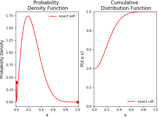
Additionally, we can plot its pdf and cdf over the interval [0,1] using the pdf() and cdf() methods:

x = np.linspace(0, 1, 1000)

fig = plt.figure()
ax1 = fig.add_subplot(1,2,1)
ax1.plot(x, rv.pdf(x), 'r-',label='exact pdf', lw=1.5)
ax1.legend(loc='upper right')
# plot probability masses at 0 and 1 as circles
ax1.plot(0.0, p*(1-q), 'ro', ms=8)
ax1.plot(1.0, p*q, 'ro', ms=8)
ax1.xlim((-0.01,1.01))
plt.xlabel('x',fontsize=12)
ax1.ylabel('Probability Density',fontsize=12)
ax1.title('Probability \n Density Function',fontsize=14)

ax2 = fig.add_subplot(1,2,2)
ax2.plot(x, rv.cdf(x), 'r',label='exact cdf', lw=1.5)
ax2.legend(loc='lower right')
ax2.xlim((-0.01,1.01))
ax2.ylim((0,1))
ax2.xlabel('x',fontsize=12)
ax2.ylabel(r'$P(X\leq x)$',fontsize=12)
ax2.title('Cumulative \n Distribution Function',fontsize=14)

fig.subplots_adjust(left=0.05, right=0.99, bottom=0.1, top=0.9,
                    wspace=0.25)

Now, we’ll generate some random variates from this distribution using the rvs() method, and plot its histogram and empirical cumulative distribution function along with the original distribution:

nsamples = 20
X = rv.rvs(nsamples) # draw random sample

ax1.hist(X,normed=True,label='sample hist',histtype='stepfilled')
ax1.legend(loc='upper right') #update legend

ax2.plot(x, beinf.ecdf(x, X), 'b',label='sample ecdf')
ax2.legend(loc='lower right')

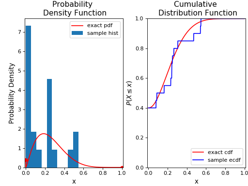
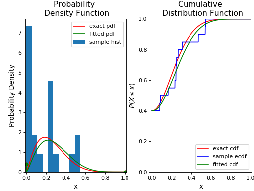
Note that we have used the ecdf() method to compute the empirical cumulative distribution function for the sample. We’ll now fit this random sample to the BEINF distribution (using fit()) and freeze a distribution object as rv_f:

a_f, b_f, p_f, q_f = beinf.fit(X)
rv_f = beinf(a_f, b_f, p_f, q_f)

Finally, we’ll plot its pdf and cdf along with the original distribution and random sample:

ax1.plot(x, rv_f.pdf(x), 'g-',label='fitted pdf', lw=1.5)
ax1.legend(loc='upper right')
ax1.plot(0.0, p_f*(1-q_f), 'go', ms=6)
ax1.plot(1.0, p_f*q_f, 'go', ms=6)

ax2.plot(x, rv_f.cdf(x), 'g',label='fitted cdf', lw=1.5)
ax2.legend(loc='lower right')   #update legend

Trend-adjusted Quantile Mapping

This section of the tutorial shows how to apply trend-adjusted quantile mapping (TAQM) using the taqm class. The methods in this class are meant to be applied to the SIC variable at an individual grid cell.

In Example 1, we’ll show how TAQM works for a grid cell for which the trend-adjusted modelled historical (TAMH) ensemble time series, the trend-adjusted observed historical (TAOH) time series, and the forecast ensemble can all be fit to the BEINF distribution (i.e. cases 1-4 described in Dirkson et al. 2018 are not encountered for any of these data samples). In Example 2, we’ll show what happens when one of cases 2-4 is encountered. In Example 3, we’ll go through a situation when case 1 is encountered (i.e. one of \(p_x=1\), \(p_y=1\), or \(p_{x_t}=1\)).

Example 1

Define the time variables relevant to calibration. The complete hindcast record is from 1981-2017 and the forecast year is 2012. The range of years \(\tau_t\) to train the TAQM calibration method is thus 1981-2011.

import numpy as np
from taqm import taqm
from scipy.stats import linregress
from beinf import beinf
import matplotlib.pyplot as plt
import os

# Time
tau_s = 1981    #start year
tau_f = 2017    #finish year
tau = np.arange(tau_s,tau_f+1)  #array of years in hindcast record

t = 2012   #forecast year
tau_t = tau[tau<t]   # only retain those years in tau which preceed the forecast year. This corresponds to TAQM-PAST in Dirkson et al

Load the model historical (MH) ensemble time series, observed historical (OH) time series, and the forecast ensemble.

os.chdir('Data')
X = np.load('MH_ex1.npy')   #load MH data
Y = np.load('OH_ex1.npy')   #load OH data
X_t = np.load('Raw_fcst_ex1.npy')   #load raw forecast
Y_t = 0.0 #made-up observation

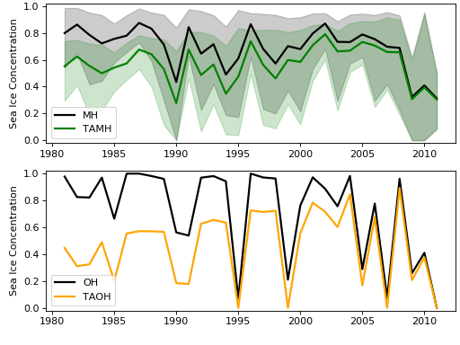
The MH and OH data loaded span the period \(\tau_t\). Now, we’ll instantiate a taqm object, and perform the trend adjustment on the MH and OH data using the trend_adjust_1p() method.

taqm = taqm()

# Get TAMH from MH
pval_x = linregress(tau_t,X.mean(axis=1))[3]  #check the p-value for MH trend over tau_t
if pval_x<0.05:
    # if significant, then adjust MH for the trend to create TAMH
    X_ta = taqm.trend_adjust_1p(X,tau_t,t)
else:
    # else, set TAMH equal to MH (i.e. don't perform the trend adjustment)
    X_ta = np.copy(X)

# Get TAOH from OH
pval_y = linregress(tau_t,Y)[3]     #check p-value for OH trend over tau_t
if pval_y<0.05:
    # if significant, then adjust OH for the trend to create TAOH
    Y_ta = taqm.trend_adjust_1p(Y,tau_t,t)
else:
    # else, set TAOH equal to OH (i.e. don't perform the trend adjustment)
    Y_ta = np.copy(Y)

The user may note that there also exists a function for performing the trend adjustment using a piece-wise linear fit of the MH and OH time series (called trend_adjust_2p()), where the breakpoint year of the piece-wise function is a user-defined input to the function (default is 1999).

The following is a plot of X and Y (top panel), and X_ta and Y_ta (bottom panel), with the ensemble range for X and X_ta encapsulated in the shaded area.

Next, we’ll fit the TAMH, TAOH, and forecast ensemble to the BEINF distribution using the fit_params() method in the taqm class:

X_ta_params, Y_ta_params, X_t_params = taqm.fit_params(X_ta,Y_ta,X_t)

Before calibrating, it’s convenient to define the variable trust_sharp_fcst, which is used to indicate what should be done when the forecast BEINF distribution has \(p_{x_t}=1\) (i.e. all ensemble members have 0% or 100% SIC). Two choices are to: (1) not calibrate (i.e. trust the raw forecast) or (2) revert to the TAOH distribution (i.e. trust the trend-adjusted climatology). For (1), set trust_sharp_fcst=True; for (2) set trust_sharp_fcst=False. For this example it doesn’t matter, because \(p_{x_t}\neq 1\), but we’ll keep this variable here as part of the general template, and set it arbitrarily to False.

# Calibrate forecast
trust_sharp_fcst = False

Now calibrate the forecast ensemble using the calibrate() method:

X_t_cal_params, X_t_cal = taqm.calibrate(X_ta_params, Y_ta_params, X_t_params,
                                                X_ta, Y_ta, X_t,trust_sharp_fcst)
print np.around(X_t_cal_params,4)
>>> [ 1.9363  6.2418  0.7129  0.    ]
print np.around(X_t_cal,4)
>>> [ inf  inf  inf  inf  inf  inf  inf  inf  inf  inf]

As described in the documentation for calibrate(), the array X_t_cal_params contains the four BEINF parameters fit to the calibrated forecast ensemble, and the X_t_cal array contains the calibrated ensemble, where in this example each value has been set to np.inf because the four BEINF distribution parameters are defined.

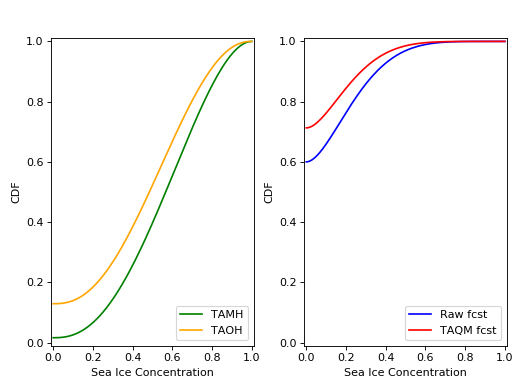
Next, we’re going to compute the SIP quantity for the raw and calibrated forecast, plot all cumulative distributions, and calculate the continuous rank probability score (CRPS) for the raw and calibrated forecast.

First, evaluate the cdf for each of these using the cdf_eval() method in the beinf class. This method handles instances when \(a\) and \(b\) aren’t known (and given the value np.inf), in which case the cdf over (0,1) is computed using the ecdf() method. When \(a\) and \(b\) are known (as is the case in this example), cdf_eval() evaluates the cdf using the cdf() method. We can also use the cdf_eval() method to compute SIP.

x = np.linspace(0, 1, 1000)
x_c = 0.15

# Evaluate cdf for the TAMH distribution at x
cdf_x_ta = beinf.cdf_eval(x, X_ta_params, X_ta)

# Evaluate cdf for the TAOH distribution at x
cdf_y_ta = beinf.cdf_eval(x, Y_ta_params, Y_ta)

# Evaluate cdf for the forecast distribution at x and calculate SIP
cdf_x_t = beinf.cdf_eval(x, X_t_params, X_t)
sip_x_t = 1.0 - beinf.cdf_eval(x_c, X_t_params, X_t)

Evaluating the cdf for the calibrated forecast ensemble is slightly more complicated than above, because we must deal with instances when either the raw forecast was “trusted” or the TAOH was “trusted” (when \(p_{x_t}=1\)). We must also deal with instances when any of \(p_{x_t}=1\), \(p_{x'}=1\), or \(p_{y'}=1\), since calibration cannot be performed. These complications can be accounted for using this if-else statement.

# first, get the p parameter for the
p_x_t = X_t_params[2] # raw forecast
p_x_ta = X_ta_params[2] # TAMH climatology
p_y_ta = Y_ta_params[2] # TAOH climatology

# Evaluate cdf for the calibrated forecast distribution at x and calculate SIP
if trust_sharp_fcst==True and p_x_t==1.0:
    # go with the original forecast data/distribution when any of the p parameters are one
    # for the three distributions used in calibration
    cdf_x_t_cal = beinf.cdf_eval(x, X_t_params, X_t)
    sip_x_t_cal = 1.0 - beinf.cdf_eval(x_c, X_t_params, X_t)
else:
    if p_x_t==1.0 or p_x_ta==1.0 or p_y_ta==1.0:
        # go with the TAOH data/distribution when any of the p parameters are
        # one for the three distributions used in calibration
        cdf_x_t_cal = beinf.cdf_eval(x, Y_ta_params, Y_ta)
        sip_x_t_cal = 1.0 - beinf.cdf_eval(x_c, Y_ta_params, Y_ta)
    else:
        # go with the calibrated forecast data/distribution
        cdf_x_t_cal = beinf.cdf_eval(x, X_t_cal_params, X_t_cal)
        sip_x_t_cal = 1.0 - beinf.cdf_eval(x_c, X_t_cal_params, X_t_cal)

Here are the cdfs for each of these distributions:

This is how we can calculate the CRPS for this forecast based on the observed value Y_t=0.0.

# Heaviside function for obs
cdf_obs = np.zeros(len(x))
cdf_obs[Y_t*np.ones(len(x))<=x] = 1.0

# CRPS for the raw forecast
crps_x_t = np.trapz((cdf_x_t - cdf_obs)**2.,x)
print crps_x_t
>>> 0.0277481871254

# CRPS for the calibrated forecast
crps_x_t_cal = np.trapz((cdf_x_t_cal - cdf_obs)**2.,x)
print crps_x_t_cal
>>> 0.0130610287303

Example 2

For a situation when one of cases 2-4 are encountered (for any of the TAMH, TAOH, or raw forecast), we’ll actually use the exact same code used in Example 1. Of course different data are loaded. In this case, the forecast distribution satisfies case 2 (all but one ensemble member are 0 or 1).

# Change directory to where the data is stored and load data
os.chdir('Data')
X = np.load('MH_ex2.npy') #load MH data
Y = np.load('OH_ex2.npy') #load OH data
X_t = np.load('Raw_fcst_ex2.npy') #load raw forecast
Y_t = 0.5   #made-up observation

By executing the same code used in Example 1, when we calibrate the forecast ensemble using the calibrate() method, we get:

X_t_cal_params, X_t_cal = taqm.calibrate(X_ta_params, Y_ta_params, X_t_params,
                                                X_ta, Y_ta, X_t,trust_sharp_fcst)
print np.around(X_t_cal_params,4)
>>> [   inf    inf  0.129  0.   ]
print np.around(X_t_cal,4)
>>> [ 0.0629     inf     inf     inf     inf     inf     inf     inf     inf
      inf]

Using the cdf_eval() (as in Example 1), the TAMH, TAOH, raw forecast, and calibrated forecast cdfs can be plotted:

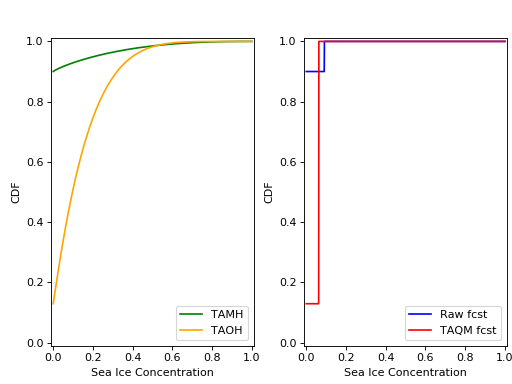
As can be seen, only the single non-0/non-1 ensemble member in X_t is quantile mapped. Additionaly, the probability \(P(X_t=0)\) has been shifted from 0.9 to 0.13 according to the bias in this probability in the TAMH ensemble time series.

The CRPS values for the raw and calibrated forecast are computed as in Example 1:

# Heaviside function for obs
cdf_obs = np.zeros(len(x))
cdf_obs[Y_t*np.ones(len(x))<=x] = 1.0

# CRPS for the raw forecast
crps_x_t = np.trapz((cdf_x_t - cdf_obs)**2.,x)
print crps_x_t
>>> 0.456351351351

# CRPS for the calibrated forecast
crps_x_t_cal = np.trapz((cdf_x_t_cal - cdf_obs)**2.,x)
print crps_x_t_cal
>>> 0.394183986276

Example 3

For a situation when case 1 is encountered for one of TAMH, TAOH, or the raw forecast, we’ll still execute the same code used in Example 1.

First however, we’ll load different data:

# Change directory to where the data is stored and load data
os.chdir('Data')
X = np.load('MH_ex3.npy') #load MH data
Y = np.load('OH_ex3.npy') #load OH data
X_t = np.load('Raw_fcst_ex3.npy') #load raw forecast
Y_t = 0.15  #made-up observation

For these particular data, both the MH and raw forecast data have \(p=1\). Because \(p_{x_t}=1\) for this example, we have the choice of trusting the raw forecast or reverting to the TAOH distribution. To show how these choices differ, we’ll first set:

trust_raw_fcst = True

The calibrated forecast parameters and values are:

X_t_cal_params, X_t_cal = taqm.calibrate(X_ta_params, Y_ta_params, X_t_params,
                                                X_ta, Y_ta, X_t,trust_sharp_fcst)
print np.around(X_t_cal_params,4)
>>> [ inf  inf   1.   0.]
print np.around(X_t_cal,4)
>>> [ inf  inf  inf  inf  inf  inf  inf  inf  inf  inf]

The cdfs for the TAMH, TAOH, raw forecast, and calibrated forecast computed using cdf_eval() can be seen in the following plot:

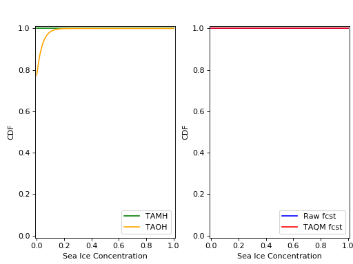
Because we have set trust_raw_fcst = True, the cdfs in the right-hand panel are identical. The CRPS values for the raw and calibrated forecast are computed as in Examples 1 and 2, and are also the same:

# Heaviside function for obs
cdf_obs = np.zeros(len(x))
cdf_obs[Y_t*np.ones(len(x))<=x] = 1.0

# CRPS for the raw forecast
crps_x_t = np.trapz((cdf_x_t - cdf_obs)**2.,x)
print crps_x_t
>>> 0.14964964965

# CRPS for the calibrated forecast
crps_x_t_cal = np.trapz((cdf_x_t_cal - cdf_obs)**2.,x)
print crps_x_t_cal
>>> 0.14964964965

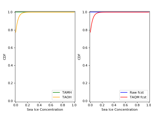
Alternatively, we could revert to the TAOH distribution by setting:

trust_raw_fcst = False

If we do this, we get the following calibrated forecast parameters and values:

X_t_cal_params, X_t_cal = taqm.calibrate(X_ta_params, Y_ta_params, X_t_params,
                                                X_ta, Y_ta, X_t,trust_sharp_fcst)
print np.around(X_t_cal_params,4)
>>> [  1.0603  26.2562   0.7742   0.    ]
print np.around(X_t_cal,4)
>>> [ inf  inf  inf  inf  inf  inf  inf  inf  inf  inf]

The plots of the cdfs for the four distributions are:

and CRPS values:

# Heaviside function for obs
cdf_obs = np.zeros(len(x))
cdf_obs[Y_t*np.ones(len(x))<=x] = 1.0

# CRPS for the raw forecast
crps_x_t = np.trapz((cdf_x_t - cdf_obs)**2.,x)
print crps_x_t
>>> 0.14964964965

# CRPS for the calibrated forecast
crps_x_t_cal = np.trapz((cdf_x_t_cal - cdf_obs)**2.,x)
print crps_x_t_cal
>>> 0.133379212736

In this particular case, we would have achieved a more skillful forecast by reverting to the TAOH distribution, and not the raw forecast.